Census data is a great resource for any GIS project, but it can be very overwhelming, and using it can be tricky at times. The data are in many forms on the Census.gov website but I have found that using the TIGER/Line with Selected Demographic and Economic Data is by far the easiest method of getting a lot out of it. This data comes in a prepackaged Geodatabase with the spatial data, a metadata table, and then many other tables with numerous attributes. Using this geodatabase is easy, but finding your story can be a little hard.
Part 1 of this 2-part post is just joining and getting a simple thematic map. Part 2 will look at creating new fields, changing numerical types, updating aliases, and getting the data ready to publish online.
Getting the Data
Let’s first go in and get our data. A quick way to find this data is to use your favorite search engine and search for census tiger with selected demographic. The first result should be the link to the data. I end up using this method because a lot of the time the census website changes the location or method to find this page.
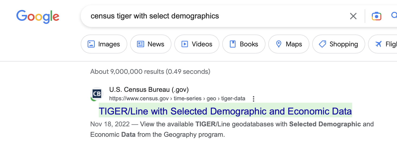
The direct link at the time of writing this post is https://www.census.gov/geographies/mapping-files/time-series/geo/tiger-data.html
(May 16, 2023)
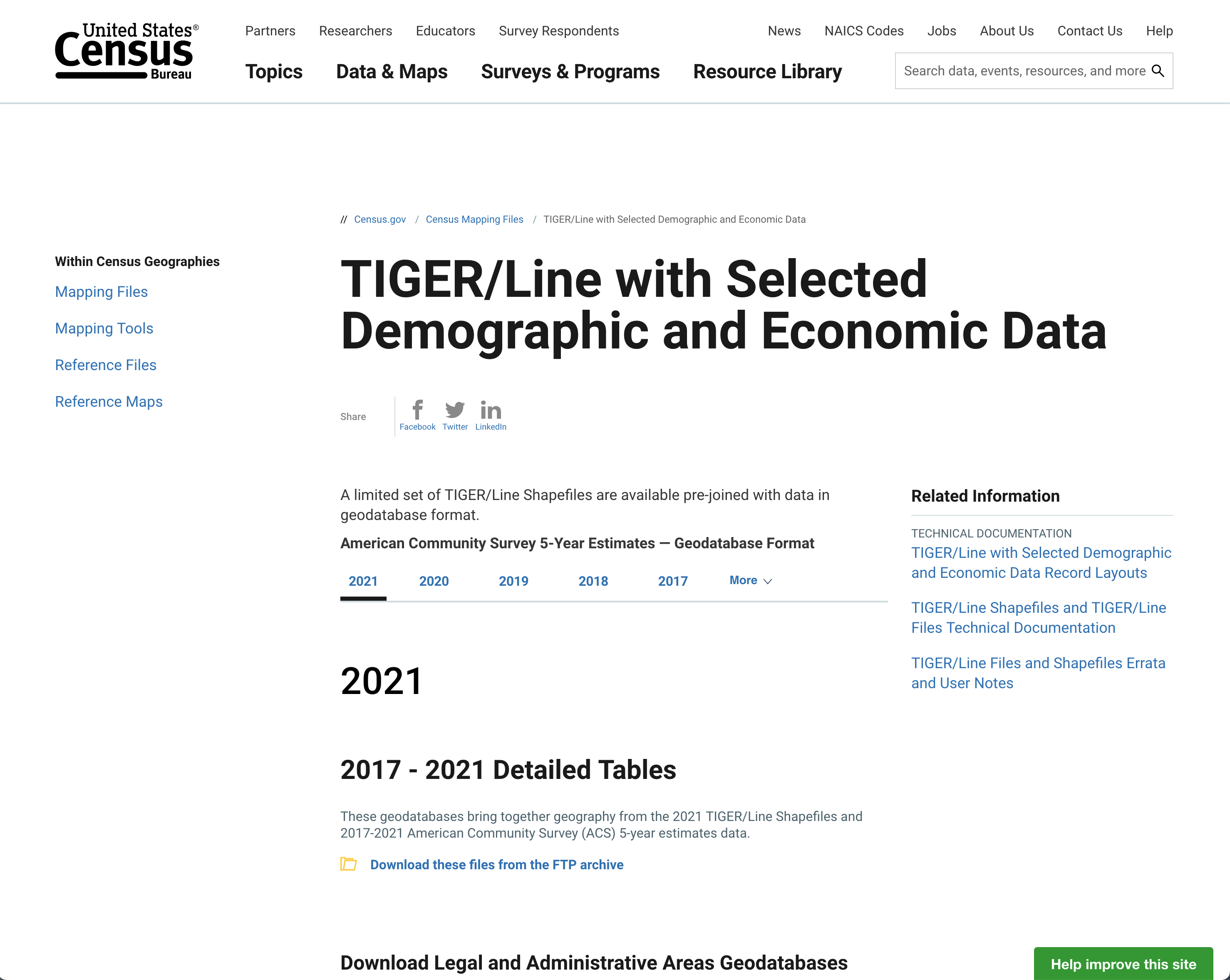
Once you are on the page you will be given a lot of options to download. The first option is the date of the data. The data included in these geodatabases are what the Census Bureau calls the long-form census or American Community Survey 5-Year Estimates. What this means it is a tally of 5 years of the American Community Surveys and are estimates based on statistical calculations from those surveys. Because of the 5 year nature of the surveys, you will see multiple years and the different years may include different attributes behind them. So your first decision is what year’s worth of data to look at.
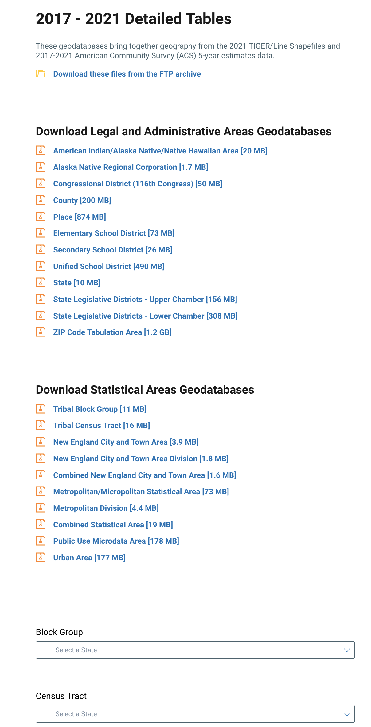
Your next decision is your geography. You will see a wide variety of geographic breakdowns for the data ranging from the state level all the way down to block groups. So for this, you will need to think about what you want to show and how detailed you want to be. For many projects, the census tract level will suffice, but you may want something different. One interesting geography you will see is ZIP Code Tabulation Area, which is a very close match to the mailing zip codes and can be used similarly. They are not exact because zip codes are created at the post office level and there is not a completely uniform layer, but this is an approximation created from mailing out the census forms.
For any layer other than the Tracts, Block Groups, and County Subdivisions there is only one download link. For the Tracts and Block Groups you will need to download the data using the dropdown to select the state.
The metadata is. at the bottom of the page (and comes with the geodatabases). This is extremely important because you cannot figure out what is in the tables and attributes with the default field names.
For this example, I am going to look at the Census Tracts for Wisconsin. Because the data are nationwide the steps will translate for all states and Census geographies, but what will change is the amount of attributes available. The Census Tracts have a great number of uses and will have tens of thousands of attributes to work with. The hardest part is to find the ones that allow you to tell the story that you want to tell.
The Geodatabase Structure
Once you download and unzip the data you will see a folder with a .GDB name. If you have that folder inside another folder with a .GDB, I would recommend moving it out so there is only one level of .GDB to prevent any read issues that you might encounter. After you have the folder all set open your favorite GIS software that can read file geodatabases. I will use ArcGIS Pro, but for Part 1, you can use QGIS and ArcMap the same way to read and join the tables.
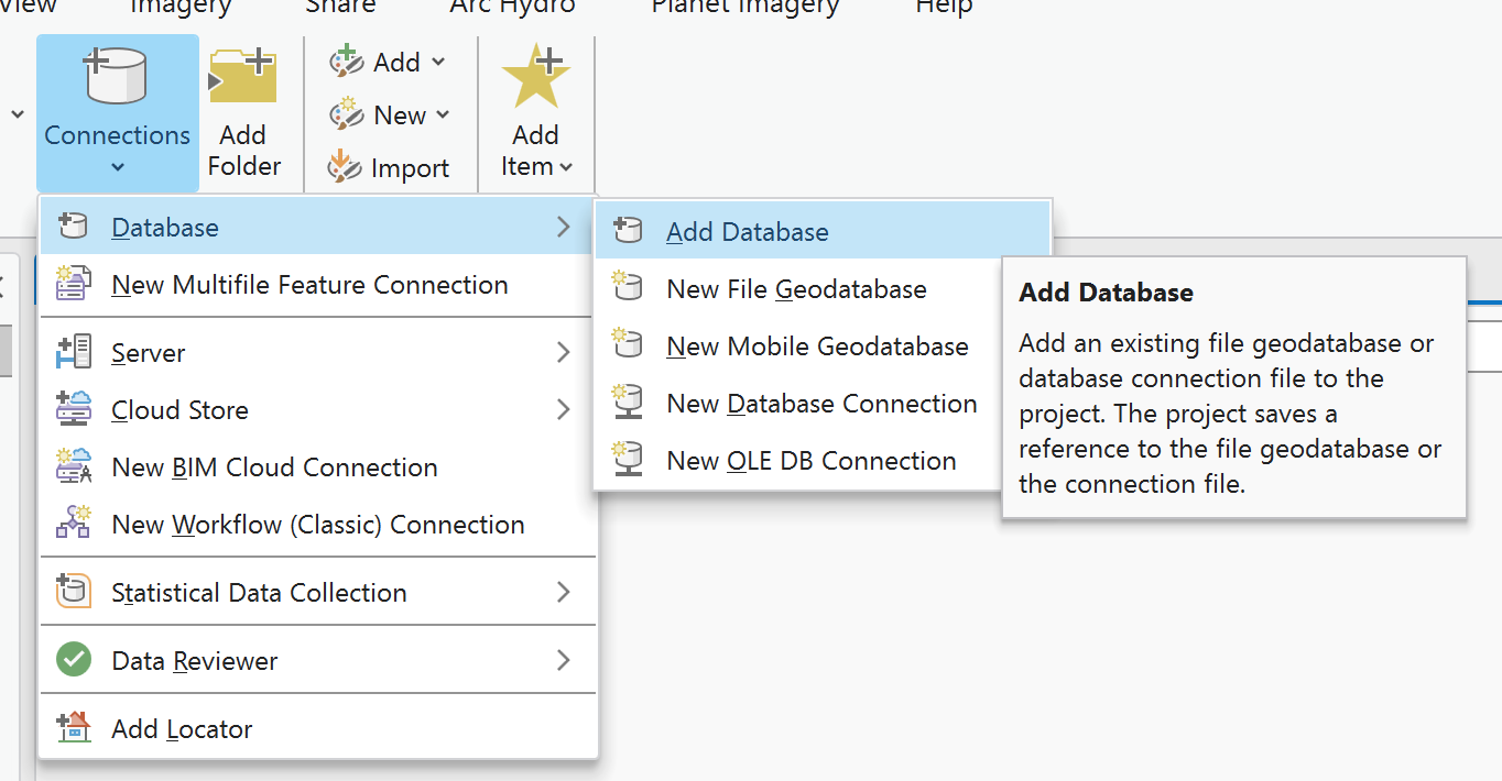
In ArcGIS Pro, I prefer to create a database link to the data so I can find it easily when working on a project. To do this go to Connections -> Database -> Add Database and then browse to your file geodatabase.
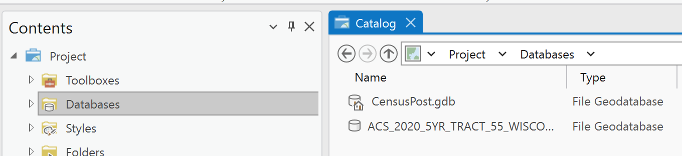
Once connected the database will be in your project databases folder.
Now that the database is connected we can open it and see the structure. You will see one Feature Class and then 31 tables. The Tract Metadata table is the same one as the documentation link from the Census page and is your key to understanding the other tables. If you downloaded a different geometry, the metadata will still be there, it will just reflect your new geometry.
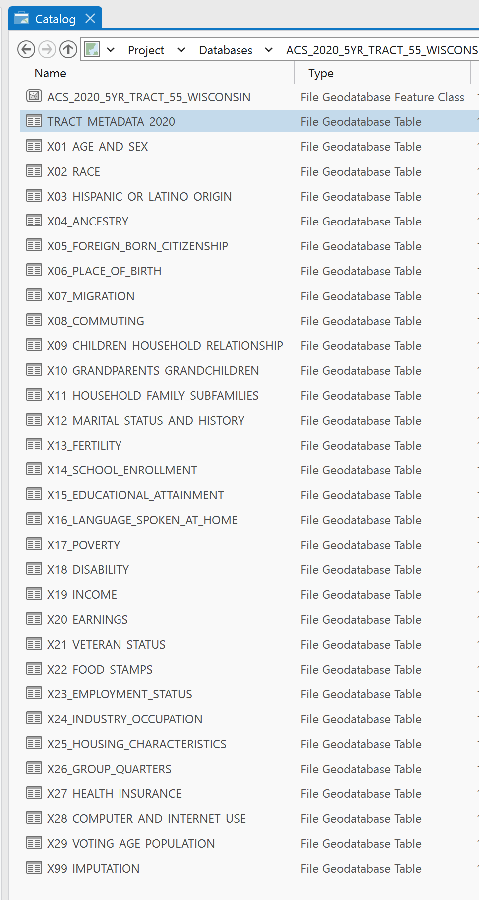
When you open the metadata table will give you a listing of attributes with their full names (aliases). When you look at the breakdown of the different tables, all of them have an x## notation, which corresponds(but does not match exactly) to the first 3 characters in the short name attributes. An example is if you want to see something from the X17 Poverty table, look for the short name of B17.
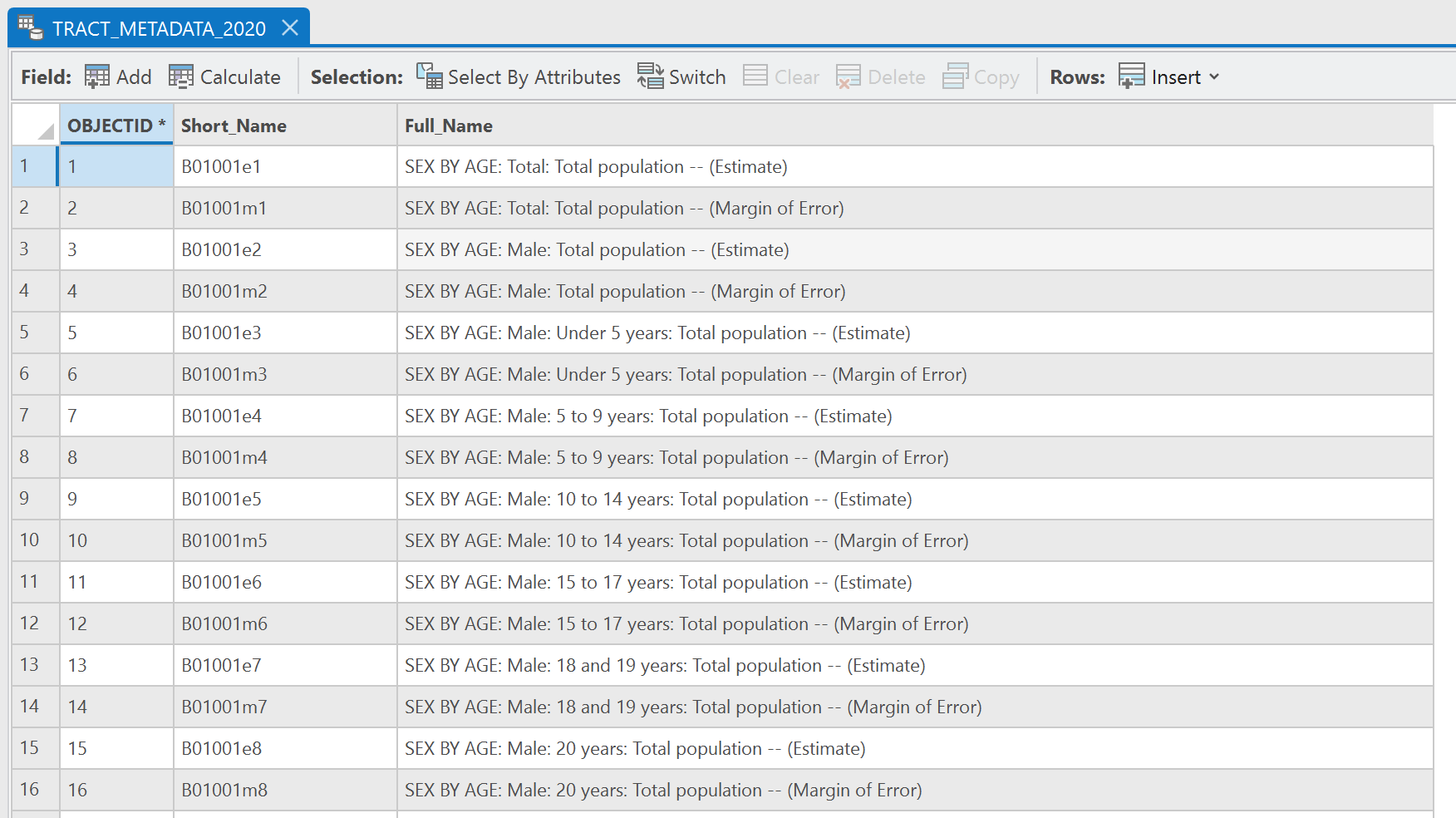
Other things you will see in the table are the estimates and margin of error (e and m) attributes. For the most part, if you are doing a thematic mapping project you will only focus on the estimates. You would use the margin of error fields when you are showing the accuracy of the ACS data, which may be good to have in a popup in an interactive map, but most of the time because of the break divisions, will not impact the thematic map.
In these attributes you will find a ton of data (just over 36.000 of them), just read the full names very carefully when picking the ones to display. The first one may not be the one that you want. For example POVERTY STATUS IN THE PAST 12 MONTHS BY SEX BY AGE: Total: Population for whom poverty status is determined — (Estimate) is not the number of people in poverty, but the total population. That field is the next one POVERTY STATUS IN THE PAST 12 MONTHS BY SEX BY AGE: Income in the past 12 months below poverty level: Population for whom poverty status is determined — (Estimate). If you want a poverty rate for each census tract, you will need to combine them and that is why it is set up that way and we will cover more on that in Part 2.

In all of the tables, there are a few key fields. In the Feature Class table, you will see a few identifying fields, the area of the land and water, and the most important field to work with this data GEOID_Data.
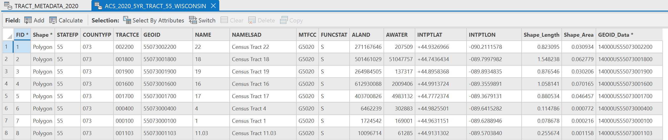
Then in all of the supplement tables, you will see the attributes that you see in the metadata and then GEOID. This GEOID field matches the GEOID_Data field and we will come back to this in a moment.
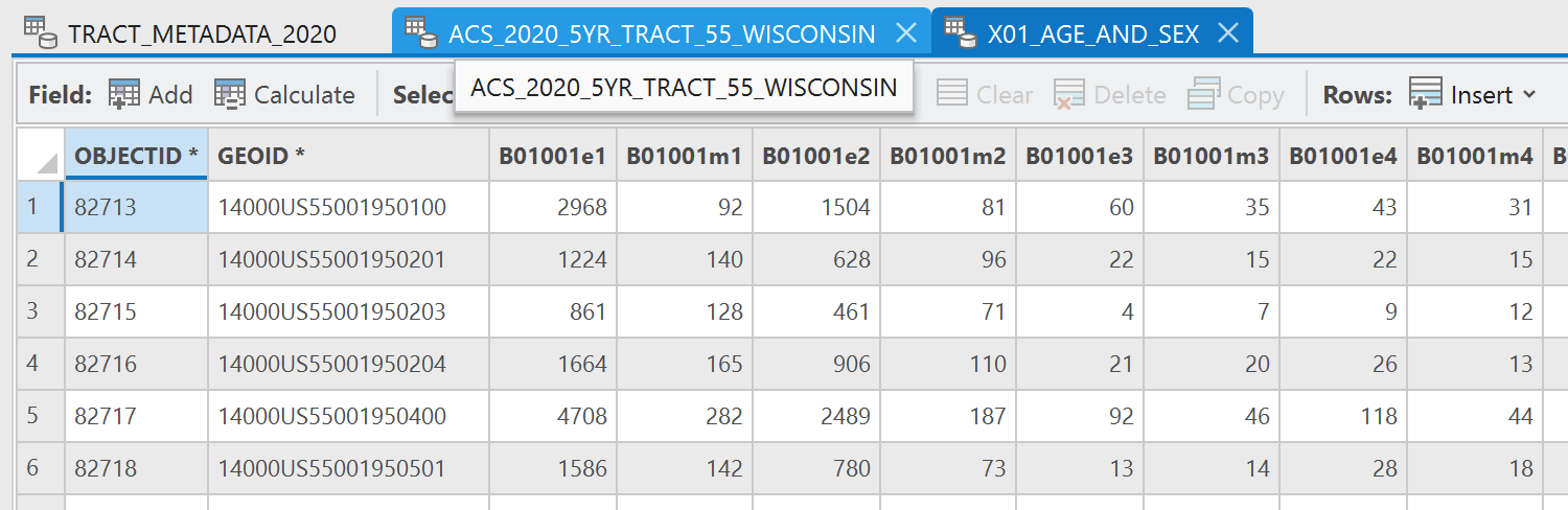
NOTE: The GEOID field in the feature class does not match the field in the supplement table.
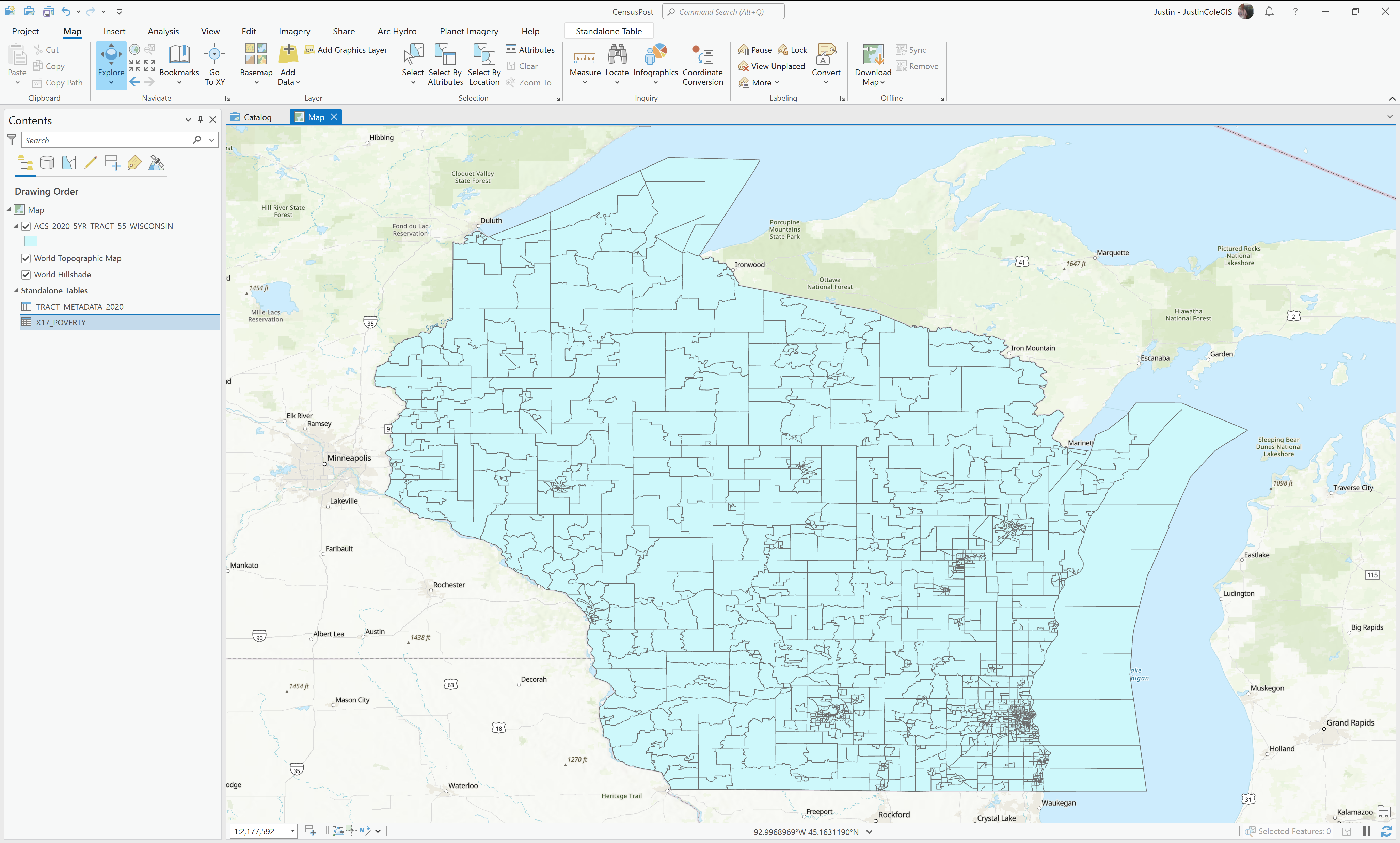
Working In GIS
So now let us change the focus from just exploring the data to making a thematic map that has good meaning. Add in the feature class, metadata table, and one table of your choosing (I am going to use Poverty).
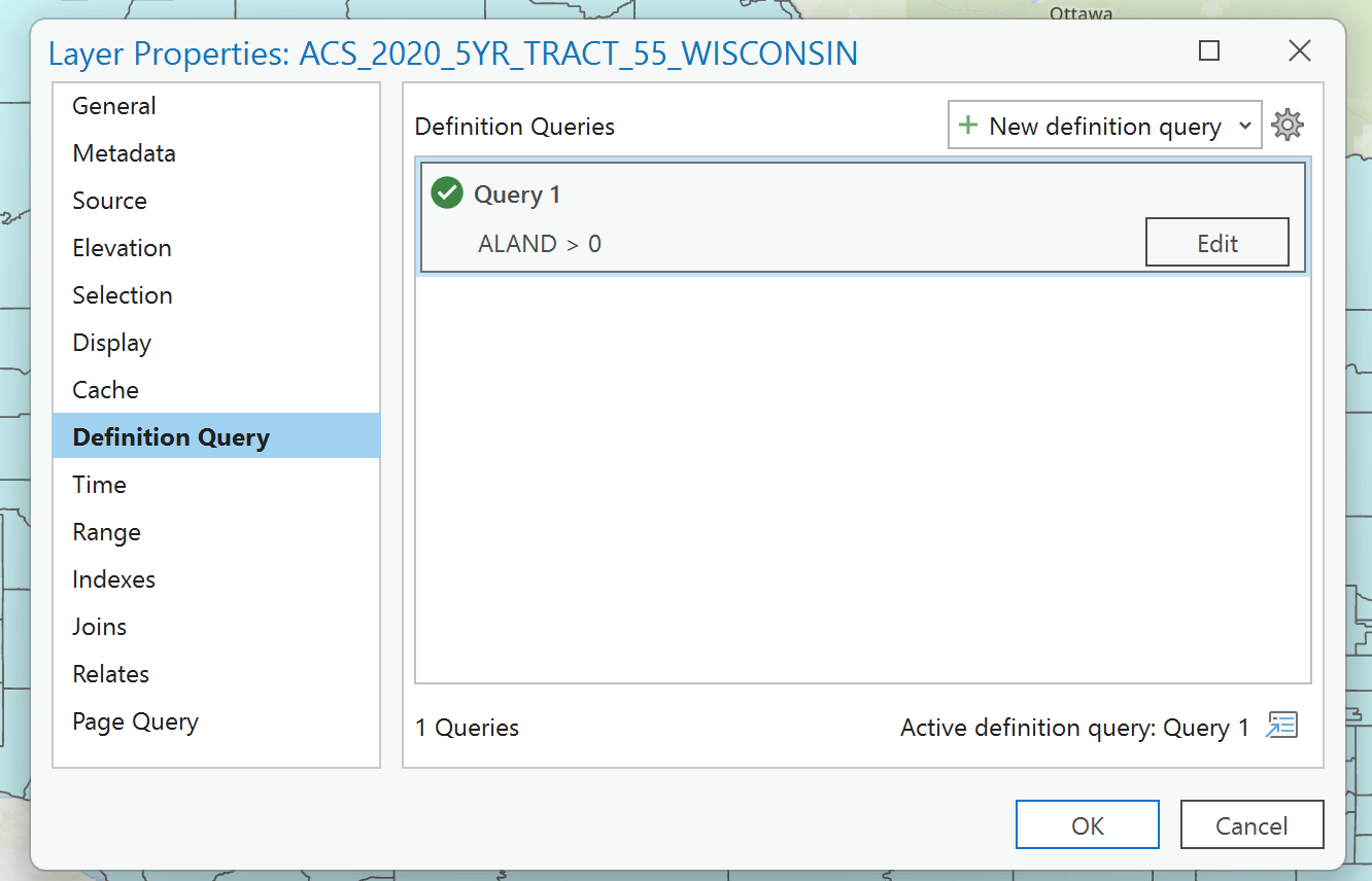
The first thing I like to do is to run a Definition Query to remove the tracts that are in the water since no one lives there. Just right-click on the feature class and go to properties. Click on the definition query tab and then set the query to ALAND > 0. This will filter out the water, but it is still a part of the data.

Now let us join the Census tract feature class to our table. Right Click the feature class and then go to Joins and Relates -> Add Join.
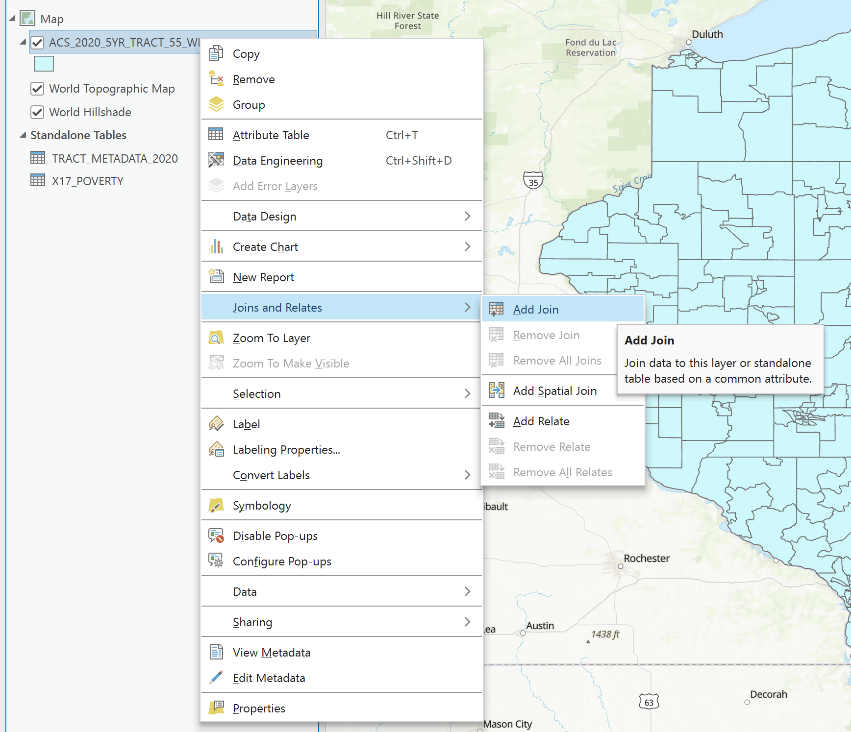
Your Input Table should be set to your Tract Feature Class and then your Join Table should be your Supplement Table (X17_Poverty in my example). Our two fields that match are GEOID_Data from the Input Table and GEOID from the Join Table. Because these tables are so large I would suggest indexing the Joined Fields. It is also good practice to always validate the join to make sure it will work. As long as you have a close match (we are filtering and that is why we do not have a 100% match) our join will work. And now click ok to join.

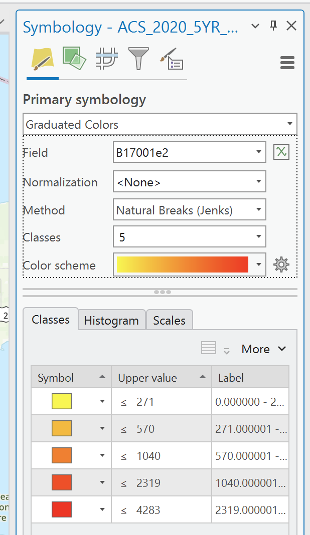
Once it is joined we can do some basic symbology to show the number of people in poverty. To do this, just go to the symbology and use a graduated color schema. Remember to pick the correct field as it will default to ALAND.

And here is where we will stop for Part 1. At this point, you can use any of the data in the supplement tables and join it to the geography to show a field. A few words of caution, do not do multiple joins on the feature class, it will make your computer run very slowly and also make it very difficult for you to work with the data with potentially thousands of fields. In Part 2, we will use the same data to make even more useful and meaningful products leveraging ArcGIS Pro’s geodatabase design tools.

One thought on ““Quick and Easy” Census Data in GIS – Part 1”